---
title: 'snRNA-seq Quality Control'
teaching: 10
exercises: 2
optional: false
---
```{r load-seurat, message=FALSE, warning=FALSE}
library(Seurat)
library(tidyverse)
library(hdf5r)
library(patchwork)
library(presto)
library(glmGamPoi)
```
```{r load-data, message=FALSE, warning=FALSE}
tissue <- c("Midbrain")
sample_names <- c("BB48", "BB49INJ", "BB50", "BB50INJ")

# Empty list to populate seurat object for each sample
list_seurat <- list()

for (sample in sample_names) {
  # Path to data directory
  data_dir <- file.path("data/ssrnaseq_data", tissue, sample)

  # Create a Seurat object for each sample
  seurat_data <- Read10X(data.dir = data_dir)
  seurat_obj <- CreateSeuratObject(
    counts = seurat_data,
    min.features = 1,
    project = paste0(tissue, "_", sample)
  )

  # Save seurat object to list
  list_seurat[[sample]] <- seurat_obj
}
```
```{r inspect-data, message=FALSE, warning=FALSE}
merged_seurat <- merge(
  x = list_seurat[[1]],
  y = list_seurat[2:length(list_seurat)],
  add.cell.id = names(list_seurat)
)

merged_seurat <- JoinLayers(merged_seurat)
merged_seurat
```
```{r}
# Check that the merged object has the appropriate sample-specific prefixes
head(merged_seurat@meta.data)
tail(merged_seurat@meta.data)
```
```{r}
merged_seurat$log10GenesPerUMI <- log10(merged_seurat$nFeature_RNA) / log10(merged_seurat$nCount_RNA)
# Create metadata dataframe
metadata <- merged_seurat@meta.data
# Add cell IDs to metadata
metadata$cells <- rownames(metadata)
# Create sample column
metadata$sample <- metadata$orig.ident
# Rename columns
metadata <- metadata %>%
dplyr::rename(
nUMI = nCount_RNA,
nGene = nFeature_RNA
)
# Add metadata back to Seurat object
merged_seurat@meta.data <- metadata
# Create .RData object to load at any time
save(merged_seurat, file = file.path("data/ssrnaseq_data/", tissue, paste0(tissue, "_merged_filtered_seurat.RData")))
```
```{r}
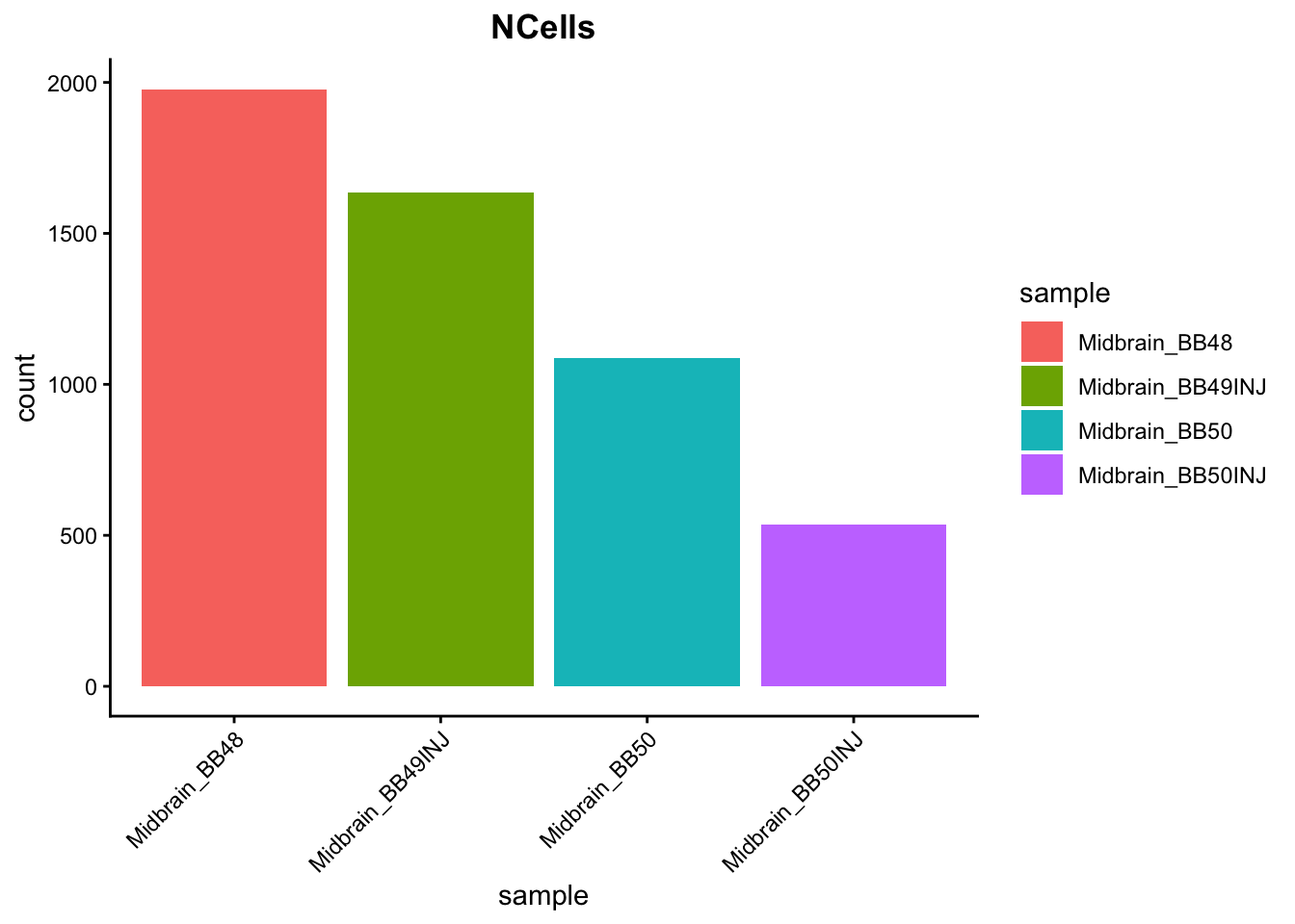
# Visualize the number of cell counts per sample
metadata %>%
ggplot(aes(x = sample, fill = sample)) +
geom_bar() +
theme_classic() +
theme(axis.text.x = element_text(angle = 45, vjust = 1, hjust = 1)) +
theme(plot.title = element_text(hjust = 0.5, face = "bold")) +
ggtitle("NCells")
```
```{r}
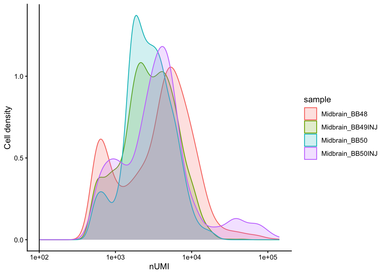
# Visualize the number UMIs/transcripts per cell
metadata %>%
ggplot(aes(color = sample, x = nUMI, fill = sample)) +
geom_density(alpha = 0.2) +
scale_x_log10() +
theme_classic() +
ylab("Cell density") +
geom_vline(xintercept = 100)
```
```{r}
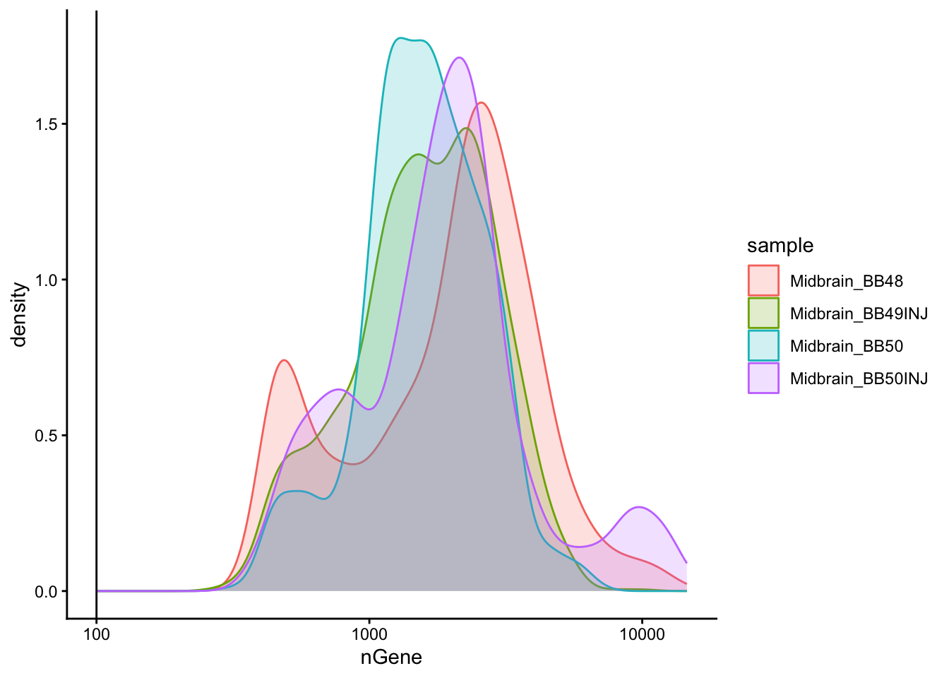
# Visualize the distribution of genes detected per cell via histogram
metadata %>%
ggplot(aes(color = sample, x = nGene, fill = sample)) +
geom_density(alpha = 0.2) +
theme_classic() +
scale_x_log10() +
geom_vline(xintercept = 100)
```
```{r}
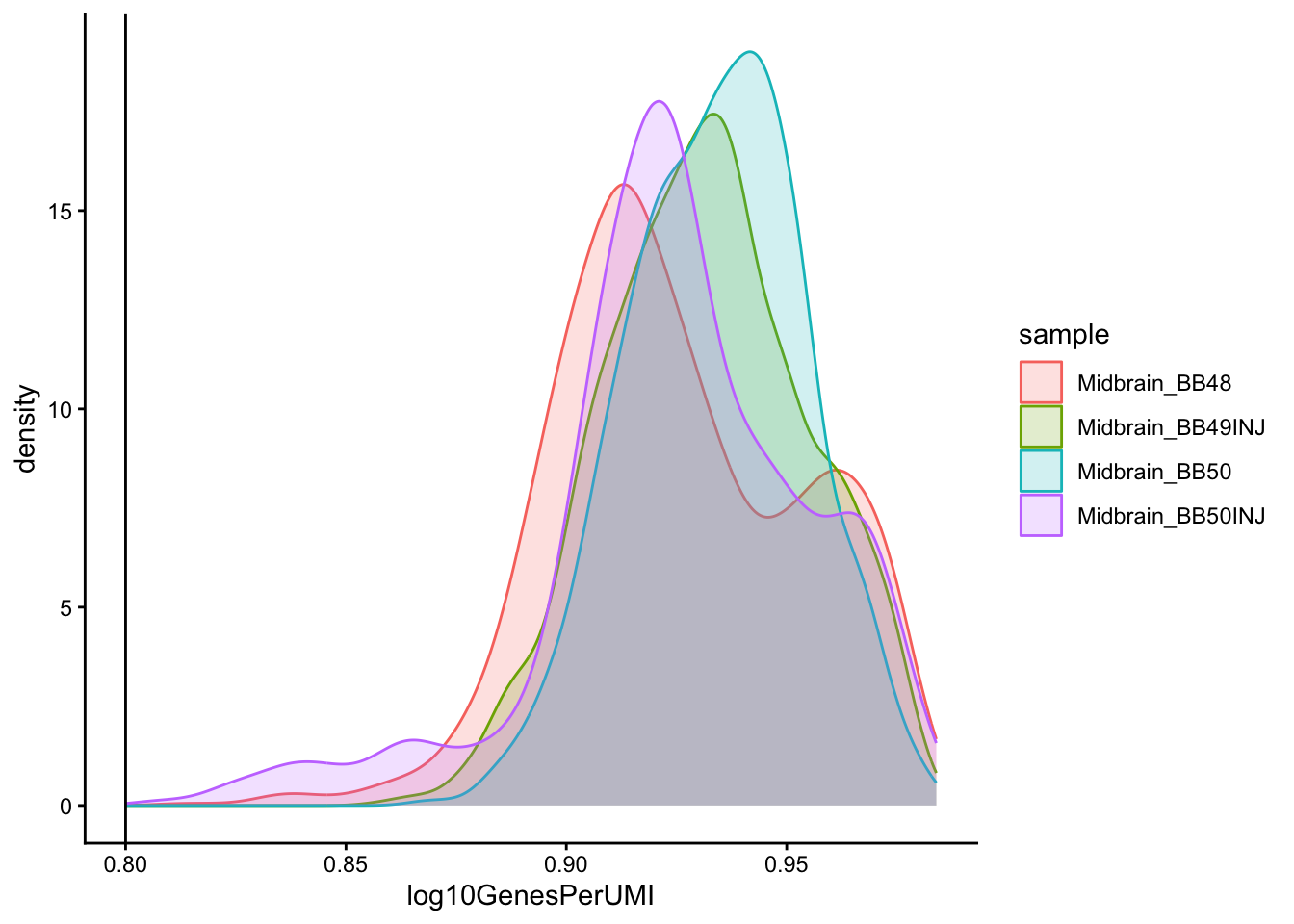
# Visualize the overall complexity of the gene expression by visualizing
# the genes detected per UMI (novelty score)
metadata %>%
ggplot(aes(x = log10GenesPerUMI, color = sample, fill = sample)) +
geom_density(alpha = 0.2) +
theme_classic() +
geom_vline(xintercept = 0.8)
```
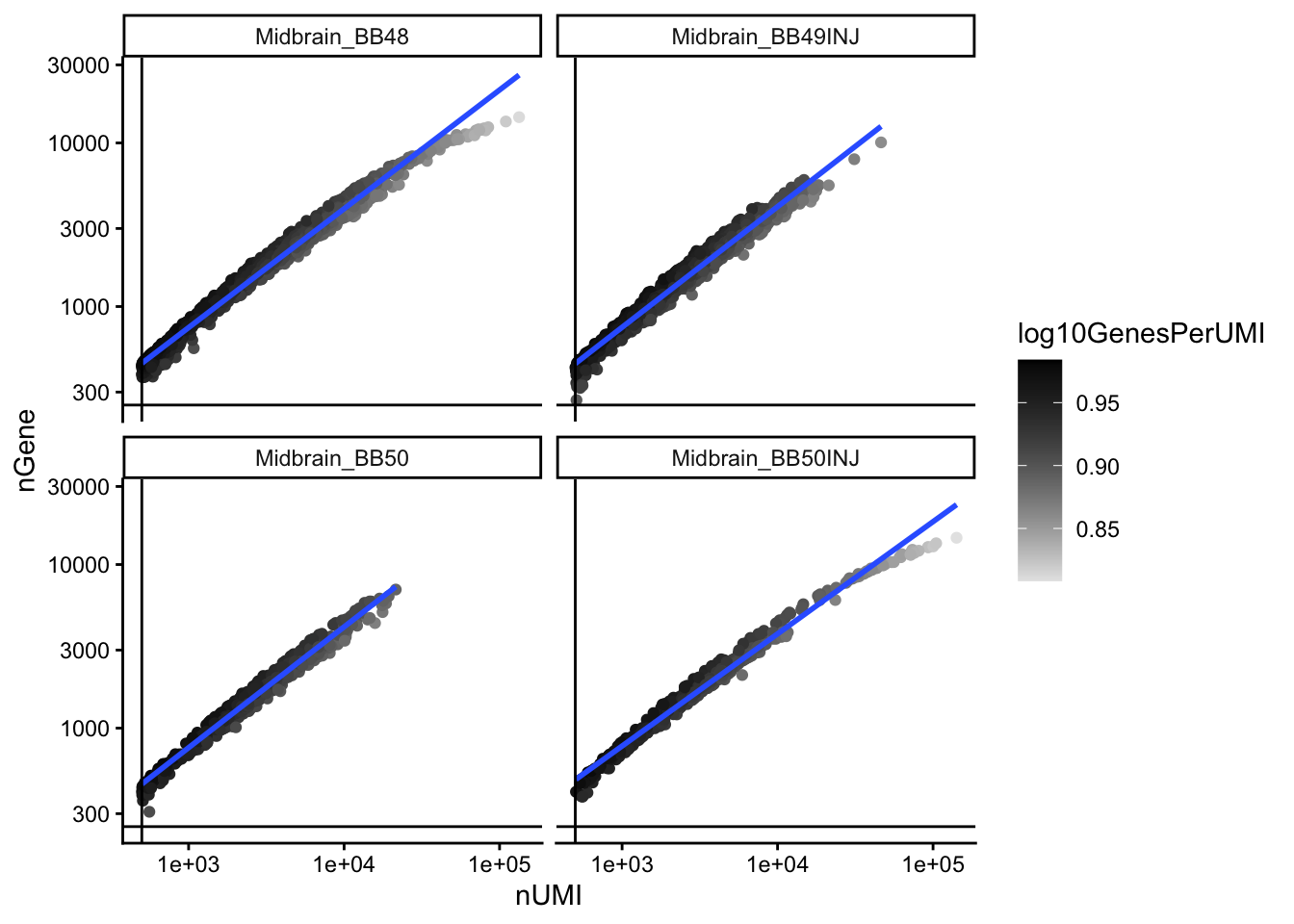
```{r,warning=FALSE}
# Visualize the correlation between genes detected and number of UMIs and
# determine whether strong presence of cells with low numbers of genes/UMIs
metadata %>%
ggplot(aes(x = nUMI, y = nGene, color = log10GenesPerUMI)) +
geom_point() +
scale_colour_gradient(low = "gray90", high = "black") +
stat_smooth(method = lm) +
scale_x_log10() +
scale_y_log10() +
theme_classic() +
geom_vline(xintercept = 500) +
geom_hline(yintercept = 250) +
facet_wrap(~sample)
```
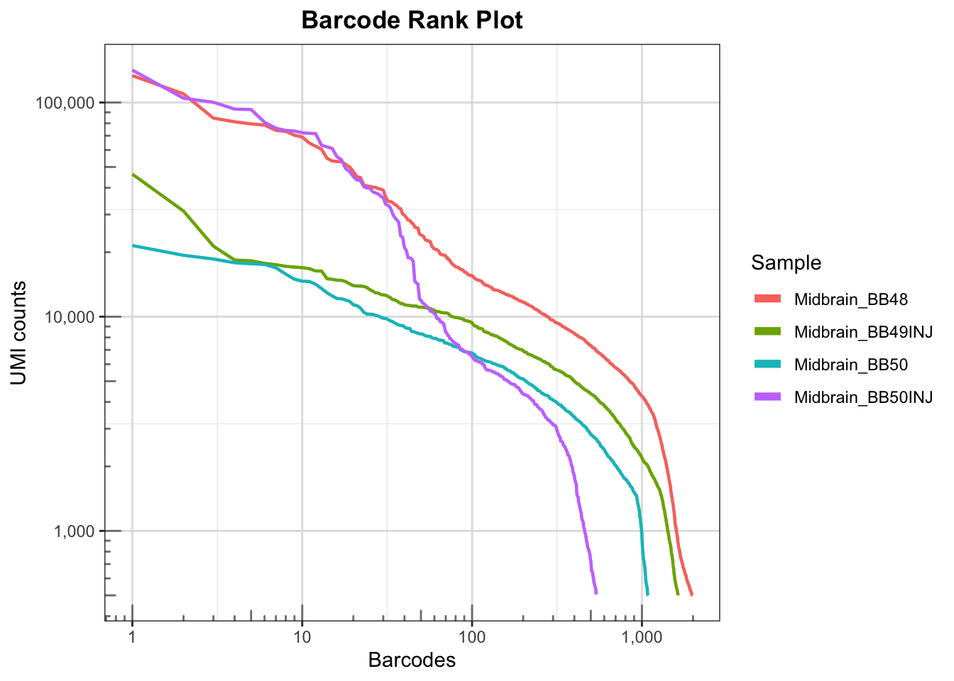
```{r barcode-rank-plot, warning=FALSE}
# Barcode rank plot (knee plot): for each sample, rank barcodes by UMI count
# (descending) and plot rank vs. UMI count on a log-log scale.
# The "knee" separates real cells (high UMI) from empty droplets (low UMI).
metadata %>%
    group_by(sample) %>%
    arrange(desc(nUMI), .by_group = TRUE) %>%
    mutate(rank = row_number()) %>%
    ungroup() %>%
    ggplot(aes(x = rank, y = nUMI, color = sample)) +
    geom_line(linewidth = 0.8) +
    scale_x_log10(labels = scales::label_comma()) +
    scale_y_log10(labels = scales::label_comma()) +
    annotation_logticks(sides = "bl", color = "grey50") +
    theme_bw() +
    theme(
        panel.grid.major = element_line(color = "grey88"),
        panel.grid.minor = element_line(color = "grey93"),
        plot.title       = element_text(hjust = 0.5, face = "bold")
    ) +
    labs(
        title = "Barcode Rank Plot",
        x     = "Barcodes",
        y     = "UMI counts",
        color = "Sample"
    ) +
    guides(color = guide_legend(override.aes = list(linewidth = 2)))
```