library(Seurat)
library(tidyverse)
library(patchwork)
library(glmGamPoi)
library(presto)
library(DESeq2)
library(limma)
library(ggrepel)
if (requireNamespace("speckle", quietly = TRUE)) library(speckle)Cell-Type Annotation and Differential Expression in the Electric Organ
NoteQuestions
- How do we turn unlabeled clusters into named cell types using curated marker genes?
- What anatomically distinguishes stalk electrocytes from face electrocytes, and how do we detect that split molecularly?
- Why is it statistically wrong to compare individual nuclei between treatment conditions, and what does pseudobulk fix?
- Does our snRNA-seq pipeline recover the gene-expression signatures of the androgen response previously found by bulk RNA-seq?
TipObjectives
- Load the post-Harmony checkpoint produced in Friday’s preprocessing episode.
- Find cluster markers with
FindAllMarkersand join NCBI gene-product descriptions for interpretation. - Assign cell-type labels (posterior/anterior face, stalk, Schwann, endothelial, satellite, immune) by scoring curated marker panels with
AddModuleScore. - Identify the innervated stalk with a falsifiable NMJ-signature prediction rather than by exclusion.
- Aggregate raw counts per (cell type × sample) and run DESeq2 with treatment as the contrast.
- Plot per-fish pseudobulk values for top DE genes and interpret the n=2-per-group result honestly.
- Cross-validate against the Losilla & Gallant 2025 bulk RNA-seq DEG table.
Introduction
Yesterday you took raw CellRanger output for four EO samples, normalized it, corrected for GEM-well batch with Harmony, and produced a clustered UMAP. The end state — saved as data/checkpoints/02_harmony_clustered.rds — is a Seurat object with unlabeled numbered clusters.
Today is the biological payoff. We assign cell-type identities to those clusters, sub-divide the electrocytes into stalk vs. face populations, and run the central statistical test of the experiment: does 11-KT change gene expression in the electric organ, and if so, in which cells and which genes?
The episode has four parts:
- Cluster markers. What genes define each cluster, and what do they tell us about cell identity?
- Cell-type annotation. Score curated marker panels and a falsifiable stalk prediction to label every cluster — splitting the electrocytes into anterior and posterior faces and an innervated stalk.
- Face validation. Confirm the posterior/anterior face split with the markers that distinguish them.
- Differential expression. Pseudobulk + DESeq2 contrast 11-KT vs. vehicle within each cell type; cross-validate against Losilla & Gallant 2025.
Setup and load Friday’s checkpoint
The checkpoint is the starting state regardless of whether you ran Friday’s full pipeline. If you finished Friday, your in-memory object should already match; loading the checkpoint guarantees a known-good entry point.
merged_seurat <- readRDS("data/checkpoints/02_harmony_clustered.rds")
merged_seurat
An object of class Seurat
50433 features across 2888 samples within 2 assays
Active assay: SCT (19912 features, 3000 variable features)
3 layers present: counts, data, scale.data
1 other assay present: RNA
4 dimensional reductions calculated: pca, umap.pca, harmony, umap.harmonyFind cluster markers
NoteThe annotator’s job
Clustering tells you which nuclei group together — it says nothing about what they are. For electric-organ tissue there is no off-the-shelf reference atlas to lean on, so we have to earn every label. The method we’ll use is the one a good detective uses: treat each cluster as a suspect, form a falsifiable prediction about its identity, score the evidence, and revise when the data disagree.
FindAllMarkers runs a Wilcoxon test for each cluster against all other cells, returning genes that distinguish each cluster from the rest. Before calling it on SCT-normalized data with multiple samples, we run PrepSCTFindMarkers() to re-correct counts to a common depth across samples.
merged_seurat <- PrepSCTFindMarkers(merged_seurat, verbose = FALSE)all_markers <- FindAllMarkers(
merged_seurat,
only.pos = TRUE,
verbose = FALSE
)
all_markers <- all_markers |>
arrange(cluster, desc(avg_log2FC))
head(all_markers, 20) p_val avg_log2FC pct.1 pct.2 p_val_adj cluster
ykt6 2.054058e-06 2.623344 0.027 0.004 4.090039e-02 0
LOC125723541 4.047744e-27 2.417031 0.147 0.027 8.059867e-23 0
napepld 1.818240e-07 2.407838 0.037 0.007 3.620479e-03 0
LOC125749277 3.282316e-35 2.355863 0.209 0.041 6.535749e-31 0
LOC125708001 1.355142e-06 2.308302 0.035 0.007 2.698359e-02 0
spa17 9.502851e-08 2.301415 0.048 0.011 1.892208e-03 0
igsf9b 9.277223e-23 2.278732 0.158 0.037 1.847281e-18 0
uhrf1 1.559386e-05 2.246374 0.029 0.006 3.105049e-01 0
LOC125719547 3.561224e-18 2.224212 0.128 0.031 7.091109e-14 0
LOC125709900 4.660350e-06 2.201387 0.032 0.007 9.279689e-02 0
LOC125747510 4.390068e-16 2.197232 0.131 0.035 8.741503e-12 0
LOC125712692 1.632575e-06 2.196333 0.037 0.008 3.250783e-02 0
il17ra1a 5.258831e-05 2.163912 0.027 0.006 1.000000e+00 0
chpfa 2.433390e-11 2.152771 0.088 0.023 4.845367e-07 0
LOC125704393 1.000116e-09 2.146210 0.064 0.015 1.991432e-05 0
LOC125712442 9.983754e-05 2.120843 0.027 0.006 1.000000e+00 0
LOC125751019 5.357706e-14 2.111445 0.102 0.025 1.066826e-09 0
kif18a 1.004328e-05 2.096798 0.035 0.008 1.999818e-01 0
hrh1 5.673328e-05 2.085909 0.029 0.007 1.000000e+00 0
kl 5.673328e-05 2.085909 0.029 0.007 1.000000e+00 0
gene
ykt6 ykt6
LOC125723541 LOC125723541
napepld napepld
LOC125749277 LOC125749277
LOC125708001 LOC125708001
spa17 spa17
igsf9b igsf9b
uhrf1 uhrf1
LOC125719547 LOC125719547
LOC125709900 LOC125709900
LOC125747510 LOC125747510
LOC125712692 LOC125712692
il17ra1a il17ra1a
chpfa chpfa
LOC125704393 LOC125704393
LOC125712442 LOC125712442
LOC125751019 LOC125751019
kif18a kif18a
hrh1 hrh1
kl klAnnotate with gene-product descriptions
The Seurat row names mix curated gene symbols and LOC##### IDs. To make the marker table interpretable, we parse the B. brachyistius GTF and join the human-readable product description for each gene.
gtf_raw <- read_tsv(
  "data/ssrnaseq_data/genes.gtf.gz",
  comment        = "#",
  col_names      = FALSE,
  col_types      = "ccciicccc",
  show_col_types = FALSE
)

gene_desc <- gtf_raw |>
  filter(str_detect(X9, 'product "')) |>
  mutate(
    gene_id   = str_extract(X9, 'gene_id "([^"]+)"', group = 1),
    gene_name = str_extract(X9, 'gene "([^"]+)"', group = 1),
    product   = str_extract(X9, 'product "([^"]+)"', group = 1)
  ) |>
  dplyr::select(gene_id, gene_name, product) |>
  distinct(gene_id, .keep_all = TRUE)

# Build a combined lookup indexed by either gene_id (LOC ID) OR gene_name (symbol)
gene_lookup <- bind_rows(
  gene_desc |> transmute(key = gene_id, gene_name, product),
  gene_desc |>
    filter(!is.na(gene_name), gene_name != gene_id) |>
    transmute(key = gene_name, gene_name, product)
) |>
  distinct(key, .keep_all = TRUE)
annotated_markers <- all_markers |>
left_join(gene_lookup |> dplyr::select(key, gene_name, product),
by = c("gene" = "key")
)
annotated_markers |>
group_by(cluster) |>
slice_max(avg_log2FC, n = 3) |>
ungroup() |>
dplyr::select(cluster, gene, gene_name, product, avg_log2FC, p_val_adj) |>
head(20)# A tibble: 20 x 6
cluster gene gene_name product avg_log2FC p_val_adj
<fct> <chr> <chr> <chr> <dbl> <dbl>
1 0 ykt6 ykt6 YKT6 v-SNARE homolog ~ 2.62 4.09e- 2
2 0 LOC125723541 LOC125723541 uncharacterized LOC12~ 2.42 8.06e-23
3 0 napepld napepld N-acyl phosphatidylet~ 2.41 3.62e- 3
4 1 LOC125741804 LOC125741804 protein shisa-6, tran~ 7.11 6.12e- 6
5 1 LOC125705310 LOC125705310 putative methyltransf~ 6.48 1.58e-12
6 1 st18 st18 ST18 C2H2C-type zinc ~ 6.31 6.12e- 6
7 2 LOC125719994 LOC125719994 uncharacterized LOC12~ 2.61 8.07e- 2
8 2 LOC125720951 LOC125720951 ankyrin repeat and SO~ 2.43 1 e+ 0
9 2 LOC125709786 LOC125709786 uncharacterized LOC12~ 2.34 1 e+ 0
10 3 LOC125725482 LOC125725482 uncharacterized LOC12~ 5.54 6.51e- 5
11 3 LOC125746231 LOC125746231 serine/threonine-prot~ 5.13 1.39e- 7
12 3 LOC125706692 LOC125706692 tyrosine-protein phos~ 4.87 4.37e- 5
13 4 LOC125738877 LOC125738877 leptin-B-like 5.36 3.18e- 3
14 4 LOC125744864 LOC125744864 tubulin alpha-1A chai~ 5.36 3.18e- 3
15 4 LOC125751762 LOC125751762 TNF receptor-associat~ 5.36 3.18e- 3
16 4 dnajb13 dnajb13 DnaJ heat shock prote~ 5.36 3.18e- 3
17 4 LOC125718053 LOC125718053 target of Myb protein~ 5.36 3.18e- 3
18 4 LOC125722975 LOC125722975 claudin-34-like, tran~ 5.36 3.18e- 3
19 5 cabp5a cabp5a calcium binding prote~ 6.40 8.33e-13
20 5 LOC125715314 LOC125715314 gamma-synuclein-like,~ 6.40 1.50e- 6
NoteWhy so many
LOC#####?
NCBI assigns LOC names as provisional symbols when a gene is computationally predicted but lacks an official name. The number is the NCBI Gene ID. The product field is where the function lives — “potassium voltage-gated channel…like” is a meaningful clue even when the gene name is LOC125743019.
For non-model genomes like B. brachyistius, this level of annotation is typical and improves over time as more papers are published.
TipExplore the markers interactively
Browse these cluster markers in the Interactive Marker-Gene Explorer: click a cluster on the UMAP to pull up its sorted, searchable marker table — the same FindAllMarkers statistics and product descriptions built above.
Annotating the clusters: predict, score, revise
Generic GO enrichment performs poorly when one cell type dominates a tissue, and the electric organ is overwhelmingly electrocyte. Instead we annotate with curated marker panels — drawn from published work on the mormyrid electric organ and from prior investigation of these exact clusters.
One discipline makes this work in a non-model organism: a feature’s name is the gene symbol only where one exists, and otherwise a provisional LOC######## ID. Never type a vertebrate symbol from memory and assume it is present — mine the product descriptions and intersect with the features you actually have. (This is why, below, the canonical “kcna7a” channel appears as LOC125743019: there is no kcna7a feature in this genome.)
Reconnaissance: who is an electrocyte?
Before splitting hairs between compartments, the first question is which clusters are even electrocyte-lineage. The principal electrogenic sodium channel scn4aa (LOC125742960) is the cleanest lineage marker.
ImportantActivity: who is an electrocyte? (6 min)
Open the Marker-Gene Explorer. In the Gene & Signature tab, single-gene mode, search scn4aa (type LOC125742960).
- Which clusters light up? Eyeball a cutoff around a per-cluster mean of ~2.5 — which clusters clear it?
- Two clusters sit just below the line (c1 ≈ 1.7, c16 ≈ 1.9) and two just above (c14 ≈ 2.7, c11 ≈ 3.0). Is 2.5 a hard boundary or a soft one?
- Now search dok2. One cluster lights up brightly. Is it an electrocyte? If not, what might it be?
TipSolution
scn4aa is high across the large electrocyte clusters (both faces and the stalk) plus the posterior-tracking c15. The 2.5 line is soft — c11/c14 sit just above, c1/c16 just below — so read it as a guide, not a gate. c16 is not an electrocyte: dok2, an immune docking protein, peaks there — it is the organ’s resident immune/myeloid population. And note scn4aa is itself only a lineage marker (detected in ≈98% of electrocytes): it tells you “electrocyte,” not which electrocyte cluster.
Curated marker panels
These panels were worked out from these exact clusters. Each is a small, positive signature we can score per nucleus.
# Gene-name discipline (see above): PMCA = LOC125738035; Kv1.7-like = LOC125743019;
# IL-8-like = LOC125720678; CCR8-like = LOC125740656; plectin-like = LOC125719088.
marker_genes <- list(
  Posterior_face = c("atp1b2b", "cdh13", "LOC125738035"),          # PMCA corroborating (weakest, ~2x)
  Stalk_NMJ      = c("musk", "chrnb1", "chrna1", "chrne"),         # post-synaptic NMJ apparatus
  Stalk_body     = c("robo2", "slit2", "sptb", "LOC125719088"),    # microstalklet + stalk-proper membrane
  Schwann        = c("col28a1a", "smoc1", "prss12", "numb"),
  Endothelial    = c("cdh5", "pecam1b", "kdr", "flt1"),
  Satellite      = c("pax7b", "notch3", "megf10", "cdh15", "myf5"),# Pax7+ progenitor pool, not muscle
  Immune         = c("dok2", "LOC125720678", "LOC125740656")
)

# Filter to genes actually present in this dataset (gene-name discipline as a safety net)
marker_genes <- lapply(marker_genes, function(g) g[g %in% rownames(merged_seurat)])
print(sapply(marker_genes, length))
Posterior_face Stalk_NMJ Stalk_body Schwann Endothelial
3 4 4 4 4
Satellite Immune
5 3 Two face programs — and why anterior is defined by absence
Each electrocyte has two electrically distinct membranes. The posterior (innervated) face carries a clean, strong program: atp1b2b (~70× enriched over the anterior face), cdh13 (~6–13×), and — more weakly — PMCA (LOC125738035, only ~2×). We lead with atp1b2b/cdh13; PMCA only corroborates.
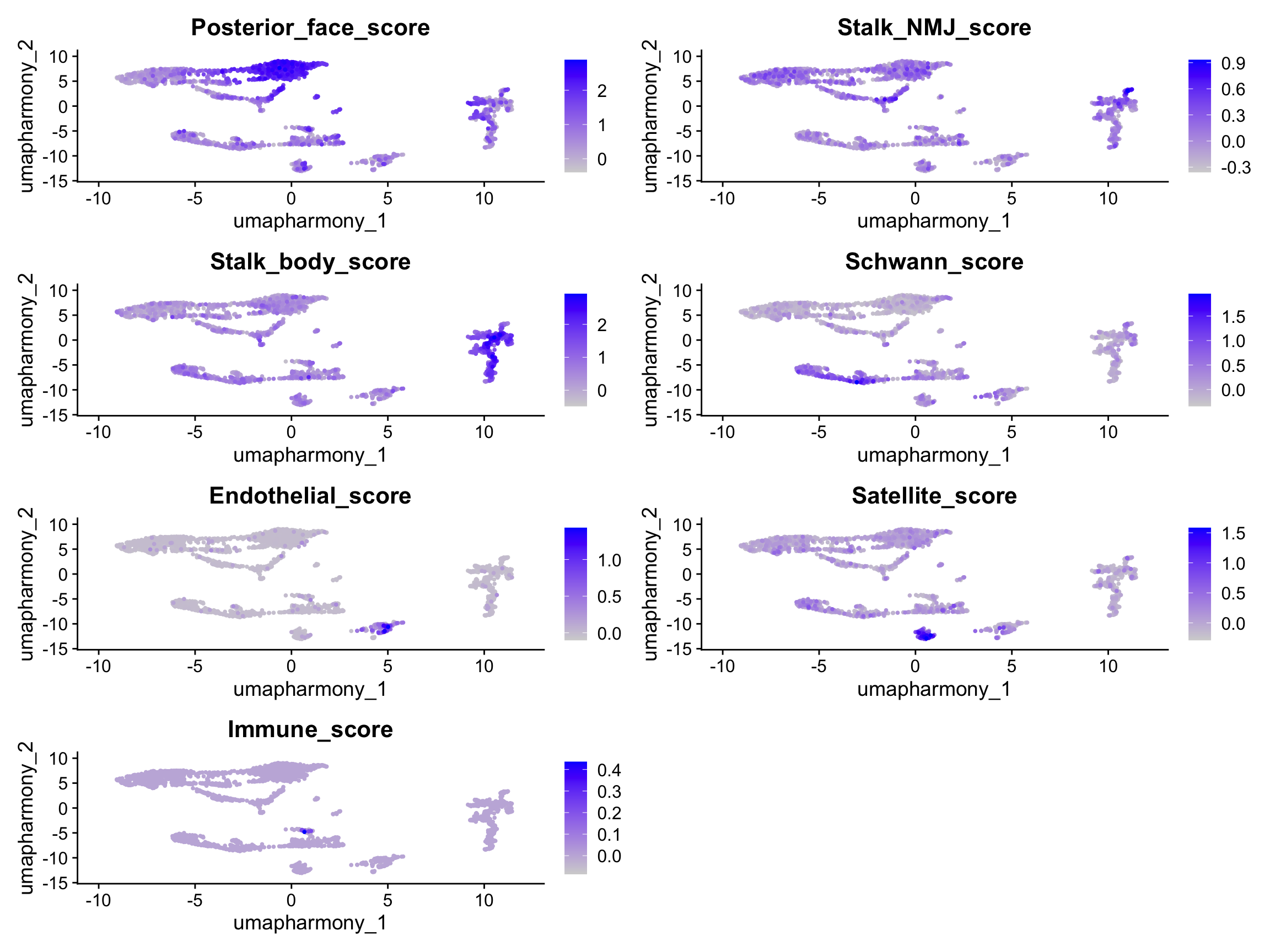
The anterior (non-innervated) face has no comparably strong positive marker. It is recognized mainly by the absence of the posterior program, with a Kv1.7-like channel (LOC125743019) weakly enriched as directional support. That is an honest limitation, not a gap in the analysis — so we score a positive Posterior_face panel and read the anterior face as the electrocyte clusters that lack it. (The polarity itself — calling the strong program posterior — rests partly on contested PMCA protein localization; that two distinct face programs exist is the solid part.)
Marker dot plot across clusters
A compact diagnostic — 3–4 most informative markers per cell type — projected as a dot plot across clusters. Dot size = fraction of cells expressing; color = mean expression.
dot_genes <- c(
  "LOC125742960", "scn4ab",                  # electrocyte lineage (Na+)
  "atp1b2b", "cdh13", "LOC125738035",        # posterior face (PMCA last = weakest)
  "LOC125743019",                            # anterior face (weak Kv1.7-like)
  "musk", "chrnb1", "chrna1", "utrn",        # stalk — NMJ
  "robo2", "slit2", "sptb",                  # stalk — body
  "col28a1a", "smoc1",                       # Schwann
  "cdh5", "pecam1b",                         # endothelial
  "pax7b", "notch3", "megf10",               # satellite
  "dok2", "LOC125720678"                     # immune
)
dot_genes <- dot_genes[dot_genes %in% rownames(merged_seurat)]

DotPlot(merged_seurat,
  features = dot_genes,
  group.by = "seurat_clusters"
) +
  RotatedAxis() +
  ggtitle("Canonical cell-type markers across clusters")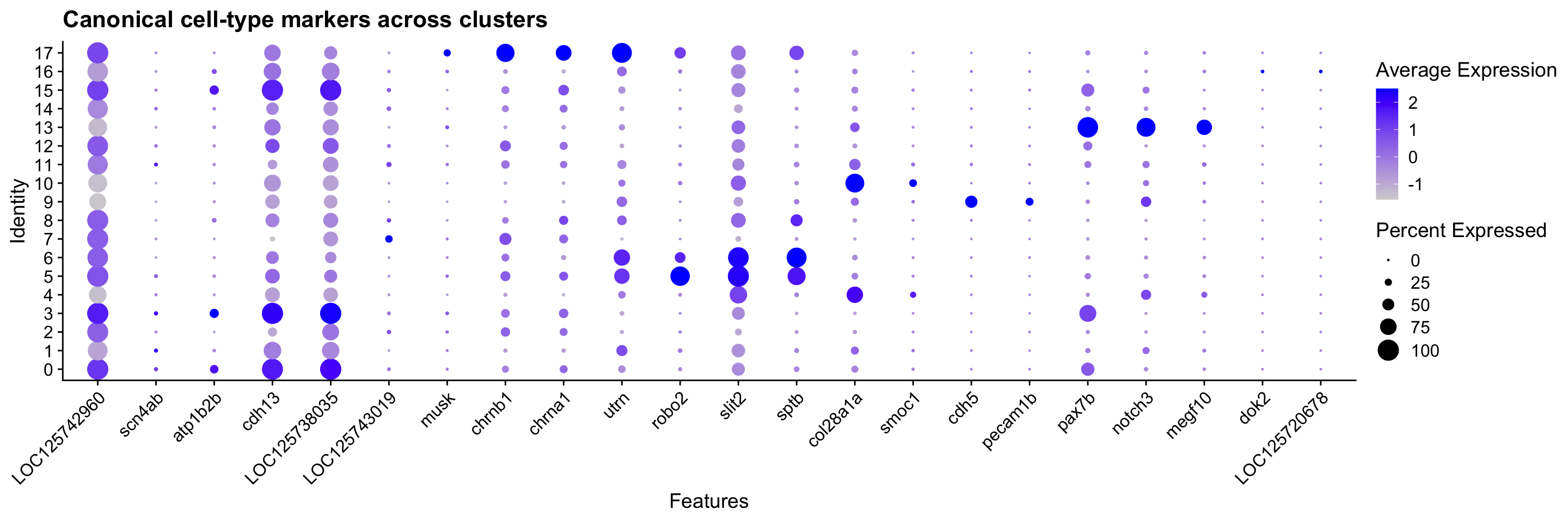
Module scores per cell type
AddModuleScore computes the average expression of a gene set minus a random control set — positive scores mean the cell expresses that gene set more than expected by chance. Pooling several markers this way is also how we rescue sparse markers: a low-copy gene like musk drops out in many nuclei even when truly on, but the panel as a whole recovers the population no single gene captures. We compute one score per panel.
for (ct in names(marker_genes)) {
  if (length(marker_genes[[ct]]) < 3) {
    message(ct, ": fewer than 3 markers found — skipping")
    next
  }
  merged_seurat <- AddModuleScore(
    merged_seurat,
    features = list(marker_genes[[ct]]),
    name     = paste0(ct, "_score"),
    nbin     = 12,
    seed     = 42
  )
  old_col <- paste0(ct, "_score1")
  new_col <- paste0(ct, "_score")
  merged_seurat@meta.data[[new_col]] <- merged_seurat@meta.data[[old_col]]
  merged_seurat@meta.data[[old_col]] <- NULL
}

score_cols <- paste0(names(marker_genes), "_score")
score_cols <- score_cols[score_cols %in% colnames(merged_seurat@meta.data)]

FeaturePlot(merged_seurat,
  features  = score_cols,
  reduction = "umap.harmony",
  ncol      = 2,
  order     = TRUE
)
Predict the stalk before you look
The tempting move is “the stalk is whatever cluster is left over after I’ve labeled the faces.” That is unfalsifiable — any leftover cluster would do. Make a positive prediction instead.
TipDefine a positive prediction
In mormyrids the stalk is the innervated compartment, so a stalk nucleus should carry the post-synaptic neuromuscular apparatus — acetylcholine-receptor subunits plus MuSK, the master organizer of the synaptic membrane. That is exactly the Stalk_NMJ panel. If no cluster carries it, we have not found the stalk — an honest result, not a failure.
ImportantActivity: predict the stalk (5 min)
In the Explorer’s Signature mode, load the predefined Stalk_NMJ set and read the per-cluster bar chart. Then switch to single-gene mode and search musk.
- Which cluster tops the NMJ signature?
- Is
muskspecific to that cluster, or spread across many? - A reasonable prior guess (before the data) was that the stalk would be cluster 12 or 14. Where do 12 and 14 actually rank?
TipSolution
Cluster 17 tops the NMJ signature decisively, and musk is essentially unique to it. The prior guess (12/14) ranks near the bottom — a falsified hypothesis, corrected by the data. c17 is small (44 nuclei, musk detected in only ~16), which is exactly why we score the whole panel rather than trust one sparse gene: each NMJ gene drops out in different nuclei, but the module score recovers the population.
We can confirm the ranking directly — average the NMJ module score within each cluster:
nmj_by_cluster <- merged_seurat@meta.data |>
  group_by(seurat_clusters) |>
  summarise(mean_NMJ = mean(Stalk_NMJ_score), n = n(), .groups = "drop") |>
  arrange(desc(mean_NMJ))
head(nmj_by_cluster, 5)
# A tibble: 5 x 3
seurat_clusters mean_NMJ n
<fct> <dbl> <int>
1 17 0.387 44
2 8 -0.0115 153
3 7 -0.0318 178
4 5 -0.0397 191
5 15 -0.0434 55stalk_cluster <- as.character(nmj_by_cluster$seurat_clusters[1]) # -> "17", the NMJ anchorCluster 17 is the NMJ / subsynaptic zone of the stalk — the electrocyte equivalent of the sole-plate nuclei that sit under a muscle synapse and run a different program from the rest of the syncytium. It does not stand alone: on the UMAP it anchors a small island (clusters 5, 6, 8, 17) set well apart from every face cluster. Clusters 5 and 6 are two stalk-body programs (microstalklets and stalk-proper, marked by robo2/slit2 and sptb/plectin); cluster 8 is a ribosomal/OXPHOS-dominated outlier the preprocessing episode flags as likely contamination, so we keep it out of the stalk.
NoteWhere are the motor neurons?
We annotate the post-synaptic side of the synapse (c17), but there is no motor-neuron cluster — and that is exactly right. A motor neuron’s soma, and therefore its nucleus, sits in the hindbrain/spinal cord; only its distal axon terminal reaches the organ. The cell body simply isn’t in the EO sample, so its absence corroborates the c17 = NMJ call rather than undercutting it. What we do capture of the neuron’s escort is the resident Schwann cells (c4/c10).
Commit the annotation
Having scored every panel and tested the stalk prediction, we can write down the cluster-to-cell-type map. This is the synthesis step: the labels are an explicit, evidence-backed decision, not the output of a fragile one-line argmax.
# Evidence-derived cluster identities.
# Faces split posterior/anterior; the stalk island (5/6/17) is merged to one label for
# downstream pseudobulk. c8 (ribosomal contamination), c1 (progenitor-like, below the
# scn4aa cutoff) and c11 (unresolved electrocyte state) are quarantined as "Other".
cluster_identity <- c(
  "0"  = "Posterior_face", "3"  = "Posterior_face", "15" = "Posterior_face",
  "2"  = "Anterior_face",  "7"  = "Anterior_face",  "12" = "Anterior_face", "14" = "Anterior_face",
  "5"  = "Stalk",          "6"  = "Stalk",          "17" = "Stalk",
  "4"  = "Schwann",        "10" = "Schwann",
  "9"  = "Endothelial",
  "13" = "Satellite",
  "16" = "Immune",
  "1"  = "Other", "8" = "Other", "11" = "Other"
)
merged_seurat$cell_type_go <- unname(
  cluster_identity[as.character(merged_seurat$seurat_clusters)]
)

# Finer view for the atlas plot: split the stalk into its NMJ vs body zones
cluster_detail <- cluster_identity
cluster_detail[c("5", "6")] <- "Stalk_body"
cluster_detail["17"]        <- "Stalk_NMJ"
merged_seurat$cell_type_detail <- unname(
  cluster_detail[as.character(merged_seurat$seurat_clusters)]
)

print(table(merged_seurat$cell_type_go))
 Anterior_face    Endothelial         Immune          Other Posterior_face
           633            143             54            538            657
     Satellite        Schwann          Stalk
112 330 421 DimPlot(merged_seurat,
reduction = "umap.harmony",
group.by = "cell_type_detail",
label = TRUE,
repel = TRUE
) +
ggtitle("EO cell types (evidence-based annotation, Harmony UMAP)") +
NoLegend()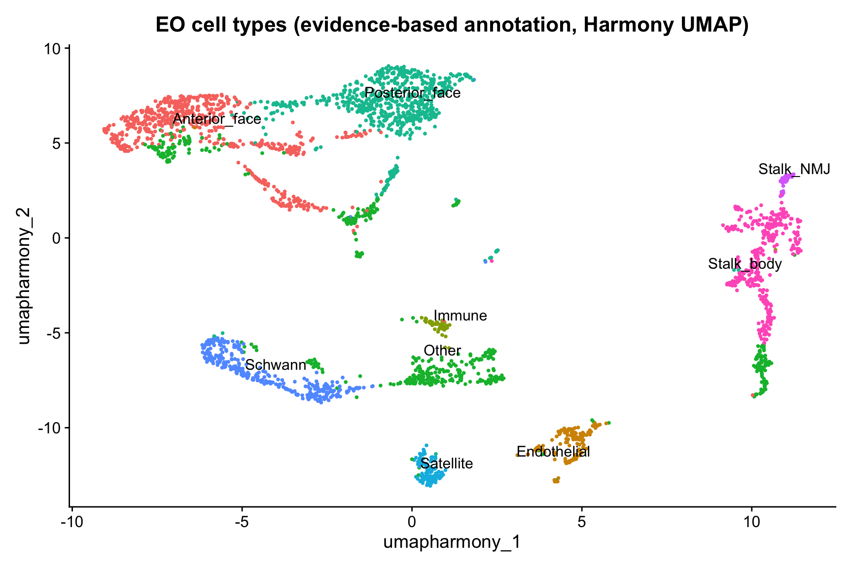
This is a natural checkpoint — the cluster-to-cell-type map is now baked into the object, and the next steps (face sub-classification + pseudobulk) build on it.
saveRDS(merged_seurat,
  file = "data/checkpoints/03_annotated.rds")
ImportantChallenge 1: Stress-test the cell-type calls (15 min)
Use the dot plot, the module-score UMAPs, and the Explorer to push back on the map we just committed.
- The stalk call. We leaned heavily on cluster 17 despite its small size. Search
muskin the Explorer: how specific is it to c17 (peak vs. everywhere else)? Given only ~16 of its 44 nuclei aremusk⁺, why is the module score still trustworthy? - The anterior face. Posterior face has
atp1b2b/cdh13; what positive marker cleanly defines the anterior face? Look at thePosterior_facemodule-score UMAP — how is the anterior face actually recognized? - A quarantined cluster. We dumped clusters 1, 8, and 11 into “Other.” Pick one, inspect its top markers in the Explorer (Tab 2), and decide: is it a real cell type we mislabeled, contamination, or genuinely unresolved? What evidence would change your mind?
TipSolution
- Stalk (c17).
muskpeaks at c17 and is near-zero elsewhere, so its specificity (the gap between pct-in and pct-out) is high even though its sensitivity is low — a classic sparse, low-copy marker. Pooling the whole NMJ panel into a module score recovers the population that any single gene misses through dropout. - Anterior face. There is no strong positive marker —
LOC125743019(Kv1.7-like) is only weakly enriched. The anterior face is the electrocyte territory that stays dark on thePosterior_facescore: it’s defined by the absence of the posterior program, which is an honest limitation of the data, not a labeling mistake. - Other (1/8/11). c8 is the ribosomal/OXPHOS outlier (~9% ribosomal, ~half from one fish) — the classic contamination signature, not a cell type. c1 sits below the
scn4aalineage cutoff with progenitor-like markers. c11 is electrocyte-lineage but has no coherent positive program — genuinely unresolved. Quarantining ambiguous clusters rather than force-labeling them is good practice: it keeps the downstream differential-expression groups clean.
TipStretch break — and a fork in the road
This is the end of the cell-type annotation block. The remaining material is denser than what came before it:
- The face sub-classification section below (markers that distinguish posterior from anterior, biology check) is conceptually optional — if you’re running short on time, skip directly to “Pseudobulk aggregation” and come back to this on your own. Anything downstream uses
cell_type_go, which is already in the saved checkpoint. - The DESeq2 + propeller + cross-study scatter sections are the central statistical payoff and should be hit live.
If you’re on pace, take five minutes to stand up, stretch, and refill your water. The rest of the episode runs straight through to differential expression.
Electrocyte face sub-classification
Optional for fast finishers — skippable if the room is tight on time. We already split the electrocytes into a posterior (innervated) face and an anterior (non-innervated) face during annotation. Here we validate that split. The posterior face generates the action potential (Nav-dominated); the anterior face generates a counter-potential. The exact channel inventory of each face is not fully resolved in B. brachyistius — our data can begin to address it.
Below we find the genes that distinguish the two labeled face groups and judge whether they form a biologically coherent program (a positive avg_log2FC means up in the posterior face).
if (all(c("Posterior_face", "Anterior_face") %in% merged_seurat$cell_type_go)) {
  face_markers <- FindMarkers(
    merged_seurat,
    ident.1  = "Posterior_face",
    ident.2  = "Anterior_face",
    group.by = "cell_type_go",
    verbose  = FALSE
  ) |>
    tibble::rownames_to_column("gene") |>
    left_join(gene_lookup |> dplyr::select(key, gene_name, product),
      by = c("gene" = "key")
    ) |>
    arrange(desc(avg_log2FC))

  head(face_markers |> filter(p_val_adj < 0.05), 15)
}
gene p_val avg_log2FC pct.1 pct.2 p_val_adj gene_name
1 agpat4 8.296955e-10 5.303864 0.058 0.000 1.652090e-05 agpat4
2 gabrb3 1.531178e-07 5.194240 0.043 0.000 3.048882e-03 gabrb3
3 LOC125708001 4.335182e-07 4.701200 0.040 0.000 8.632213e-03 LOC125708001
4 LOC125718202 3.622391e-16 4.683278 0.108 0.003 7.212905e-12 LOC125718202
5 LOC125723541 4.902664e-22 4.660558 0.149 0.005 9.762185e-18 LOC125723541
6 pde4d 1.636650e-163 4.507246 0.896 0.205 3.258898e-159 pde4d
7 fgf2 9.346464e-43 4.500901 0.294 0.016 1.861068e-38 fgf2
8 LOC125746073 3.032220e-113 4.471916 0.840 0.314 6.037756e-109 LOC125746073
9 LOC125717831 4.449973e-56 4.398700 0.394 0.033 8.860786e-52 LOC125717831
10 cpm 8.083820e-39 4.372577 0.275 0.017 1.609650e-34 cpm
11 sema3fb 6.757699e-28 4.372577 0.205 0.014 1.345593e-23 sema3fb
12 st6galnac2 3.682897e-36 4.324824 0.251 0.013 7.333385e-32 st6galnac2
13 atp1b2b 7.433356e-49 4.314382 0.336 0.021 1.480130e-44 atp1b2b
14 LOC125716348 1.603324e-63 4.300929 0.432 0.036 3.192538e-59 LOC125716348
15 mfsd2b 5.065399e-33 4.268240 0.233 0.013 1.008622e-28 mfsd2b
product
1 1-acylglycerol-3-phosphate O-acyltransferase 4 (lysophosphatidic acid acyltransferase, delta)
2 gamma-aminobutyric acid type A receptor subunit beta3, transcript variant X1
3 uncharacterized LOC125708001
4 ATP-citrate synthase-like, transcript variant X2
5 uncharacterized LOC125723541, transcript variant X1
6 phosphodiesterase 4D, cAMP-specific, transcript variant X8
7 fibroblast growth factor 2
8 multiple C2 and transmembrane domain-containing protein 1-like
9 ras-related protein Rab-26-like, transcript variant X2
10 carboxypeptidase M, transcript variant X2
11 sema domain, immunoglobulin domain (Ig), short basic domain, secreted, (semaphorin) 3Fb
12 ST6 (alpha-N-acetyl-neuraminyl-2,3-beta-galactosyl-1,3)-N-acetylgalactosaminide alpha-2,6-sialyltransferase 2
13 ATPase Na+/K+ transporting subunit beta 2b
14 polyamine-transporting ATPase 13A3-like, transcript variant X3
15 major facilitator superfamily domain containing 2B, transcript variant X2if (exists("face_markers")) {
face_markers |>
filter(p_val_adj < 0.05, abs(avg_log2FC) > 0.5, !is.na(product)) |>
mutate(product = as.character(product),
category = case_when(
str_detect(product, regex("potassium|sodium|calcium|chloride|channel|transporter", ignore_case = TRUE)) ~ "Ion channel/transporter",
str_detect(product, regex("collagen|fibronectin|laminin|cadherin|integrin", ignore_case = TRUE)) ~ "ECM/adhesion",
str_detect(product, regex("kinase|phosphatase|GTPase|signaling", ignore_case = TRUE)) ~ "Signaling",
str_detect(product, regex("actin|myosin|tubulin|spectrin|cytoskeletal", ignore_case = TRUE)) ~ "Cytoskeletal",
str_detect(product, regex("receptor|ligand", ignore_case = TRUE)) ~ "Receptor/ligand",
TRUE ~ "Other/uncharacterized"
)) |>
dplyr::count(category, sort = TRUE)
} category n
1 Other/uncharacterized 919
2 Signaling 145
3 Cytoskeletal 66
4 Receptor/ligand 60
5 ECM/adhesion 36
6 Ion channel/transporter 25
NoteThree reasons electrocyte clusters can split
When non-stalk electrocyte clusters form two UMAP-separated groups, the explanation is usually one of three things:
- Biological — anterior vs. posterior face identity. The posterior face is dominated by Nav channels; the anterior face relies on K⁺ and Ca²⁺ channels. Coherent ion-channel families in the top DEGs support this.
- Spatial/anatomical — rostral vs. caudal segments. Some mormyrids show regional EO specialization. Cytoskeletal or ECM differences (not channels) hint at this.
- Technical — residual sample-of-origin effects. Even after Harmony, mild batch can split a cell type. Check sample composition per cluster.
Rule of thumb: many between-group DEGs in coherent functional families → biological. Few DEGs or uncharacterized proteins → likely technical.
Pseudobulk differential expression with DESeq2
This is the central analytical question of the workshop: does 11-KT change gene expression in the electric organ?
Why pseudobulk: the pseudoreplication problem
This dataset contains ~2,900 nuclei from four fish — two 11-KT (BB48, BB49INJ), two vehicle (BB50, BB50INJ). A tempting but wrong approach is to test each nucleus as an independent observation: Wilcoxon on ~1,400 11-KT nuclei vs. ~1,400 vehicle nuclei.
The problem: nuclei from the same fish are not independent. They share fish-level variation in diet, microbiome, stress history, and countless other factors that have nothing to do with 11-KT. Treating each nucleus as a replicate inflates the degrees of freedom ~700-fold, deflates p-values accordingly, and lets results from one unusual fish look like a reproducible treatment effect.
Pseudobulk solves this: we sum raw counts per gene across nuclei within each (cell type × sample), producing one count per gene per cell type per fish. DESeq2 then models those four numbers per cell type with treatment as the contrast.
WarningRaw counts only — never SCT residuals or Harmony
DESeq2 fits its own size-factor normalization internally. It requires raw integer count data:
| Input | Appropriate for DE? |
|---|---|
AggregateExpression(assay = "RNA") |
✅ Yes — raw UMI counts |
SCT residuals (scale.data) |
❌ No — continuous, not integer |
Log-normalized counts (data slot) |
❌ No — violates count model |
| Harmony-corrected embeddings | ❌ No — not counts at all |
Use assay = "RNA" in every AggregateExpression call. SCT and Harmony are for clustering and visualization only.
Build the pseudobulk matrix
pseudobulk_counts <- AggregateExpression(
  merged_seurat,
  assays        = "RNA",
  group.by      = c("cell_type_go", "orig.ident"),
  return.seurat = FALSE
)$RNA

cat("Pseudobulk matrix dimensions:", dim(pseudobulk_counts), "\n")
Pseudobulk matrix dimensions: 30521 32 print(colnames(pseudobulk_counts)) [1] "Anterior-face_EO-BB48" "Anterior-face_EO-BB49INJ"
[3] "Anterior-face_EO-BB50" "Anterior-face_EO-BB50INJ"
[5] "Endothelial_EO-BB48" "Endothelial_EO-BB49INJ"
[7] "Endothelial_EO-BB50" "Endothelial_EO-BB50INJ"
[9] "Immune_EO-BB48" "Immune_EO-BB49INJ"
[11] "Immune_EO-BB50" "Immune_EO-BB50INJ"
[13] "Other_EO-BB48" "Other_EO-BB49INJ"
[15] "Other_EO-BB50" "Other_EO-BB50INJ"
[17] "Posterior-face_EO-BB48" "Posterior-face_EO-BB49INJ"
[19] "Posterior-face_EO-BB50" "Posterior-face_EO-BB50INJ"
[21] "Satellite_EO-BB48" "Satellite_EO-BB49INJ"
[23] "Satellite_EO-BB50" "Satellite_EO-BB50INJ"
[25] "Schwann_EO-BB48" "Schwann_EO-BB49INJ"
[27] "Schwann_EO-BB50" "Schwann_EO-BB50INJ"
[29] "Stalk_EO-BB48" "Stalk_EO-BB49INJ"
[31] "Stalk_EO-BB50" "Stalk_EO-BB50INJ" Sample metadata for the design matrix
Parse the column names ("CellType_EO-BB48" etc.) into a metadata data frame with treatment as a factor — vehicle as reference so positive log2FC means up in 11-KT.
pb_meta <- data.frame(
  col_id = colnames(pseudobulk_counts),
  stringsAsFactors = FALSE
) |>
  tidyr::separate(col_id,
    into  = c("cell_type", "orig_ident"),
    sep   = "_",
    extra = "merge"
  ) |>
  mutate(
    # AggregateExpression sanitizes "_" in group labels to "-"; restore underscores so
    # cell_type matches the annotation-side labels (Posterior_face, Anterior_face, ...).
    cell_type = gsub("-", "_", cell_type),
    sample = sub("EO-", "", orig_ident),
    treatment = case_when(
      sample %in% c("BB48", "BB49INJ") ~ "11kt",
      TRUE ~ "vehicle"
    ),
    treatment = factor(treatment, levels = c("vehicle", "11kt"))
  )

rownames(pb_meta) <- colnames(pseudobulk_counts)
pb_meta
cell_type orig_ident sample treatment
Anterior-face_EO-BB48 Anterior_face EO-BB48 BB48 11kt
Anterior-face_EO-BB49INJ Anterior_face EO-BB49INJ BB49INJ 11kt
Anterior-face_EO-BB50 Anterior_face EO-BB50 BB50 vehicle
Anterior-face_EO-BB50INJ Anterior_face EO-BB50INJ BB50INJ vehicle
Endothelial_EO-BB48 Endothelial EO-BB48 BB48 11kt
Endothelial_EO-BB49INJ Endothelial EO-BB49INJ BB49INJ 11kt
Endothelial_EO-BB50 Endothelial EO-BB50 BB50 vehicle
Endothelial_EO-BB50INJ Endothelial EO-BB50INJ BB50INJ vehicle
Immune_EO-BB48 Immune EO-BB48 BB48 11kt
Immune_EO-BB49INJ Immune EO-BB49INJ BB49INJ 11kt
Immune_EO-BB50 Immune EO-BB50 BB50 vehicle
Immune_EO-BB50INJ Immune EO-BB50INJ BB50INJ vehicle
Other_EO-BB48 Other EO-BB48 BB48 11kt
Other_EO-BB49INJ Other EO-BB49INJ BB49INJ 11kt
Other_EO-BB50 Other EO-BB50 BB50 vehicle
Other_EO-BB50INJ Other EO-BB50INJ BB50INJ vehicle
Posterior-face_EO-BB48 Posterior_face EO-BB48 BB48 11kt
Posterior-face_EO-BB49INJ Posterior_face EO-BB49INJ BB49INJ 11kt
Posterior-face_EO-BB50 Posterior_face EO-BB50 BB50 vehicle
Posterior-face_EO-BB50INJ Posterior_face EO-BB50INJ BB50INJ vehicle
Satellite_EO-BB48 Satellite EO-BB48 BB48 11kt
Satellite_EO-BB49INJ Satellite EO-BB49INJ BB49INJ 11kt
Satellite_EO-BB50 Satellite EO-BB50 BB50 vehicle
Satellite_EO-BB50INJ Satellite EO-BB50INJ BB50INJ vehicle
Schwann_EO-BB48 Schwann EO-BB48 BB48 11kt
Schwann_EO-BB49INJ Schwann EO-BB49INJ BB49INJ 11kt
Schwann_EO-BB50 Schwann EO-BB50 BB50 vehicle
Schwann_EO-BB50INJ Schwann EO-BB50INJ BB50INJ vehicle
Stalk_EO-BB48 Stalk EO-BB48 BB48 11kt
Stalk_EO-BB49INJ Stalk EO-BB49INJ BB49INJ 11kt
Stalk_EO-BB50 Stalk EO-BB50 BB50 vehicle
Stalk_EO-BB50INJ Stalk EO-BB50INJ BB50INJ vehicleRun DESeq2 per cell type
For each cell type with at least 2 samples per condition, build a DESeqDataSet and extract results for the 11-KT vs. vehicle contrast.
sample_counts_per_ct <- pb_meta |>
  group_by(cell_type, treatment) |>
  summarise(n = n(), .groups = "drop") |>
  group_by(cell_type) |>
  filter(all(n >= 2)) |>
  pull(cell_type) |>
  unique() |>
  setdiff("Other")   # "Other" pools contamination/ambiguous clusters — not a biological group

cat("Cell types testable:\n")
Cell types testable:print(sample_counts_per_ct)[1] "Anterior_face" "Endothelial" "Immune" "Posterior_face"
[5] "Satellite" "Schwann" "Stalk" de_results <- list()
dds_objects <- list()
for (ct in sample_counts_per_ct) {
cols <- which(pb_meta$cell_type == ct)
mat <- pseudobulk_counts[, cols, drop = FALSE]
meta_sub <- pb_meta[cols, , drop = FALSE]
mat <- mat[rowSums(mat) > 0, , drop = FALSE]
dds <- DESeqDataSetFromMatrix(
countData = mat,
colData = meta_sub,
design = ~treatment
)
suppressWarnings(dds <- DESeq(dds, quiet = TRUE))
res <- results(dds,
contrast = c("treatment", "11kt", "vehicle"),
alpha = 0.05
)
de_results[[ct]] <- as.data.frame(res) |>
tibble::rownames_to_column("gene") |>
mutate(cell_type = ct) |>
arrange(padj)
dds_objects[[ct]] <- dds
}
de_combined <- bind_rows(de_results)
cat("Total gene × cell-type tests:", nrow(de_combined), "\n")Total gene <U+00D7> cell-type tests: 121553 saveRDS(list(de_results = de_results, dds_objects = dds_objects, pb_meta = pb_meta),
file = "data/checkpoints/04_pseudobulk_dds.rds")
WarningInterpreting DESeq2 with n=2 per group
With only 2 biological replicates per condition, DESeq2 borrows statistical strength across genes via shrinkage, but uncertainty stays high:
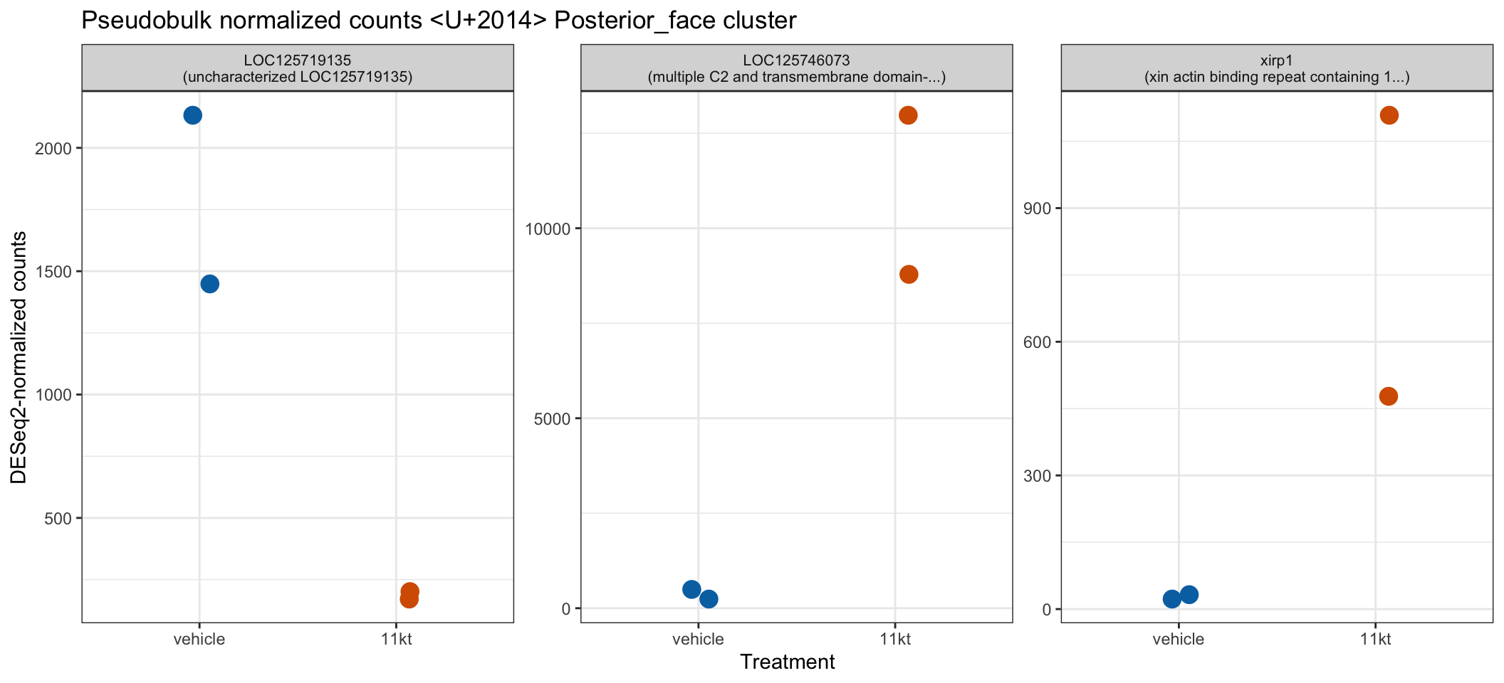
- Focus on log2FoldChange magnitude and direction, not just padj. A gene where both 11-KT fish are higher than both vehicle fish is more credible than one driven by a single outlier.
- Padj values will be large — many genes will not reach 0.05. This is the correct result for an n=2 experiment, not a problem to fix.
- A dispersion warning is expected with n=2 — DESeq2 can’t robustly estimate dispersion from two points and borrows from the genome-wide trend.
- Treat the output as a ranked list for follow-up, not a definitive call of DE genes.
Top DE genes per cell type
de_combined |>
  filter(!is.na(padj), padj < 0.1) |>
  group_by(cell_type) |>
  slice_min(padj, n = 5) |>
  ungroup() |>
  left_join(gene_lookup |> dplyr::select(key, product), by = c("gene" = "key")) |>
  dplyr::select(cell_type, gene, product, log2FoldChange, lfcSE, padj)
# A tibble: 23 x 6
cell_type gene product log2FoldChange lfcSE padj
<chr> <chr> <chr> <dbl> <dbl> <dbl>
1 Anterior_face LOC125751819 cytosolic carboxyp~ 4.92 0.537 1.91e-16
2 Anterior_face xirp1 xin actin binding ~ 5.14 0.575 8.17e-16
3 Anterior_face pdzrn3b PDZ domain contain~ 3.98 0.458 4.62e-15
4 Anterior_face rnf207b ring finger protei~ 3.05 0.406 6.00e-11
5 Anterior_face LOC125745822 uncharacterized LO~ -2.75 0.371 9.17e-11
6 Endothelial LOC125746073 multiple C2 and tr~ 4.28 0.804 1.62e- 3
7 Endothelial LOC125747551 myosin heavy chain~ 2.54 0.557 3.97e- 2
8 Posterior_face LOC125746073 multiple C2 and tr~ 4.84 0.394 5.01e-31
9 Posterior_face xirp1 xin actin binding ~ 4.88 0.527 5.18e-17
10 Posterior_face LOC125719135 uncharacterized LO~ -3.28 0.381 1.30e-14
# i 13 more rowsPer-fish pseudobulk visualization
With n=2 per group, never plot means ± SE — show every fish’s value as a point. The point of pseudobulk is biological-replicate-level evidence; the visualization should reflect that.
ct_vis <- if ("Posterior_face" %in% sample_counts_per_ct) "Posterior_face" else sample_counts_per_ct[1]

dds_vis <- dds_objects[[ct_vis]]
dds_vis <- estimateSizeFactors(dds_vis)
norm_mat <- counts(dds_vis, normalized = TRUE)

top_genes <- de_results[[ct_vis]] |>
  filter(!is.na(padj), padj < 1) |>
  slice_min(padj, n = 3) |>
  pull(gene)

norm_tidy <- norm_mat[top_genes, , drop = FALSE] |>
  as.data.frame() |>
  tibble::rownames_to_column("gene") |>
  pivot_longer(-gene, names_to = "col_id", values_to = "norm_count") |>
  left_join(pb_meta |> tibble::rownames_to_column("col_id"), by = "col_id") |>
  left_join(gene_lookup |> dplyr::select(key, gene_name, product),
    by = c("gene" = "key")
  ) |>
  mutate(
    label = if_else(is.na(product) | product == "",
      gene,
      paste0(gene, "\n(", str_trunc(product, 40), ")")
    )
  )

ggplot(norm_tidy, aes(x = treatment, y = norm_count, color = treatment)) +
  geom_point(size = 4, position = position_jitter(width = 0.08, seed = 42)) +
  facet_wrap(~label, scales = "free_y", nrow = 1) +
  scale_color_manual(values = c("11kt" = "#D55E00", "vehicle" = "#0072B2")) +
  theme_bw() +
  theme(legend.position = "none", strip.text = element_text(size = 8)) +
  labs(
    title = paste("Pseudobulk normalized counts —", ct_vis, "cluster"),
    y     = "DESeq2-normalized counts",
    x     = "Treatment"
  )
ImportantChallenge 2: Pick a gene and defend it (15 min)
From the per-fish dot plot, choose one top DE gene that you’d present in a lab meeting as a candidate 11-KT-responsive gene.
- Are both 11-KT fish higher (or both lower) than both vehicle fish? If not, the effect rides on one fish — say so plainly.
- Look up the
productdescription. Does the gene’s function make biological sense in the context of EOD lengthening? - What would you do next to validate this candidate?
TipSolution
There’s no single right answer. The honest reasoning chain:
- Step 1: Replicate consistency. If 11-KT fish #1 and #2 sit clearly above (or below) vehicle fish #1 and #2, the effect is reproducible across animals. If one 11-KT fish overlaps a vehicle fish, the result is fragile — one more animal could flip it.
- Step 2: Biological plausibility. Genes encoding ion channels (Na⁺, K⁺, Ca²⁺), sarcomeric proteins, or known androgen-pathway components are biologically credible candidates. Lipid-metabolism genes are often systemic androgen responses.
- Step 3: Validation. qPCR on independent fish; in situ hybridization to confirm cell-type specificity; published 11-KT response data from related work (you’ll do exactly this in the next section against Losilla & Gallant 2025).
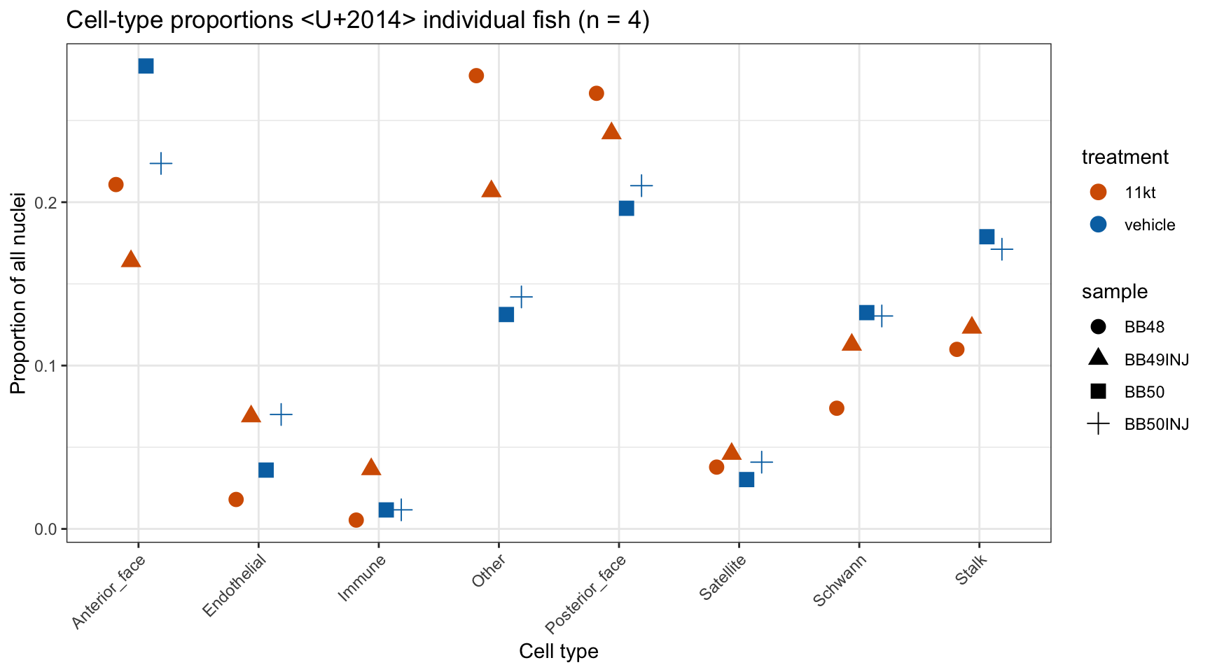
Differential cell-type abundance
Beyond which genes change, we can ask whether cell-type proportions shift. If 11-KT drives the satellite pool to differentiate into electrocytes, the Satellite fraction should shrink and the face populations grow.
prop_table <- merged_seurat@meta.data |>
  group_by(orig.ident, cell_type_go, treatment, sample) |>
  summarise(n_cells = n(), .groups = "drop") |>
  group_by(orig.ident) |>
  mutate(total = sum(n_cells), prop = n_cells / total) |>
  ungroup()

prop_table |>
  dplyr::select(sample, treatment, cell_type_go, n_cells, total, prop) |>
  arrange(treatment, cell_type_go)
# A tibble: 32 x 6
sample treatment cell_type_go n_cells total prop
<chr> <chr> <chr> <int> <int> <dbl>
1 BB48 11kt Anterior_face 117 555 0.211
2 BB49INJ 11kt Anterior_face 157 958 0.164
3 BB48 11kt Endothelial 10 555 0.0180
4 BB49INJ 11kt Endothelial 66 958 0.0689
5 BB48 11kt Immune 3 555 0.00541
6 BB49INJ 11kt Immune 35 958 0.0365
7 BB48 11kt Other 154 555 0.277
8 BB49INJ 11kt Other 198 958 0.207
9 BB48 11kt Posterior_face 148 555 0.267
10 BB49INJ 11kt Posterior_face 232 958 0.242
# i 22 more rowsggplot(prop_table,
aes(x = cell_type_go, y = prop, color = treatment, shape = sample)
) +
geom_point(size = 3.5, position = position_dodge(width = 0.5)) +
scale_color_manual(values = c("11kt" = "#D55E00", "vehicle" = "#0072B2")) +
theme_bw() +
theme(axis.text.x = element_text(angle = 45, hjust = 1)) +
labs(
title = "Cell-type proportions — individual fish (n = 4)",
y = "Proportion of all nuclei",
x = "Cell type"
)
Test for differential abundance (propeller or arcsine-limma fallback)
Both propeller and the arcsine-limma fallback apply an arcsine-square-root transform to proportions before fitting a linear model. With n=2 per group the power is low — report direction and magnitude, not p-values alone.
if (requireNamespace("speckle", quietly = TRUE)) {
  prop_results <- speckle::propeller(
    clusters = merged_seurat$cell_type_go,
    sample   = merged_seurat$orig.ident,
    group    = merged_seurat$treatment
  )
  print(prop_results)
} else {
  message("speckle not available; using arcsine-limma fallback")

  prop_wide <- prop_table |>
    mutate(asin_prop = asin(sqrt(prop))) |>
    dplyr::select(orig.ident, treatment, cell_type_go, asin_prop) |>
    pivot_wider(
      id_cols     = c(orig.ident, treatment),
      names_from  = cell_type_go,
      values_from = asin_prop,
      values_fill = 0
    ) |>
    arrange(treatment)

  design <- model.matrix(~treatment, data = prop_wide)
  ct_cols <- setdiff(names(prop_wide), c("orig.ident", "treatment"))
  fit <- limma::lmFit(t(prop_wide[, ct_cols]), design)
  fit <- limma::eBayes(fit)
  da_res <- limma::topTable(fit, coef = 2, n = Inf)
  print(da_res)
}
BaselineProp.clusters BaselineProp.Freq PropMean.11kt
Other Other 0.18628809 0.24207903
Stalk Stalk 0.14577562 0.11654159
Schwann Schwann 0.11426593 0.09330437
Posterior_face Posterior_face 0.22749307 0.25441893
Anterior_face Anterior_face 0.21918283 0.18734695
Satellite Satellite 0.03878116 0.04188343
Endothelial Endothelial 0.04951524 0.04345577
Immune Immune 0.01869806 0.02096993
PropMean.vehicle PropRatio Tstatistic P.Value FDR
Other 0.13663304 1.7717459 3.2991167 0.03138478 0.1774371
Stalk 0.17503401 0.6658226 -2.9330839 0.04435927 0.1774371
Schwann 0.13137719 0.7102022 -1.7871595 0.15071707 0.2503546
Posterior_face 0.20320006 1.2520613 1.7774505 0.15240593 0.2503546
Anterior_face 0.25356341 0.7388564 -1.7545432 0.15647160 0.2503546
Satellite 0.03552674 1.1789269 0.8595603 0.43993323 0.5865776
Endothelial 0.05302178 0.8195835 -0.6163723 0.57199669 0.6537105
Immune 0.01164378 1.8009557 0.3269088 0.76062280 0.7606228Validation: cross-study comparison with Losilla & Gallant 2025
Our pseudobulk result is more trustworthy if it independently recovers the gene-expression changes Losilla & Gallant (2025) found by bulk RNA-seq under 17α-methyltestosterone treatment. We expect: same direction of regulation for shared hits, and a positive correlation in effect sizes.
losilla_bulk <- read_csv(
  "data/ssrnaseq_data/EO/losilla_et_al_data.csv",
  show_col_types = FALSE
) |>
  dplyr::rename(
    gene_bulk  = "Gene Symbol",
    desc_bulk  = "Gene Description",
    logFC_bulk = "logFC",
    FDR_bulk   = "FDR"
  ) |>
  mutate(direction_bulk = if_else(logFC_bulk > 0, "up (androgen)", "down (androgen)"))

cat("Losilla & Gallant 2025 bulk DEGs:", nrow(losilla_bulk), "\n")
Losilla & Gallant 2025 bulk DEGs: 245 ct_check <- if ("Posterior_face" %in% names(de_results)) "Posterior_face" else names(de_results)[1]
overlap_tbl <- de_results[[ct_check]] |>
inner_join(losilla_bulk, by = c("gene" = "gene_bulk")) |>
mutate(
direction_snrna = if_else(log2FoldChange > 0, "up (11-KT)", "down (11-KT)"),
concordant = sign(log2FoldChange) == sign(logFC_bulk)
) |>
left_join(gene_lookup |> dplyr::select(key, gene_name, product), by = c("gene" = "key"))
n_detected <- nrow(overlap_tbl)
n_concordant <- sum(overlap_tbl$concordant, na.rm = TRUE)
cat(sprintf(
"Losilla DEGs detected in %s pseudobulk: %d / %d (%.0f%%)\n",
ct_check, n_detected, nrow(losilla_bulk),
100 * n_detected / nrow(losilla_bulk)
))Losilla DEGs detected in Posterior_face pseudobulk: 198 / 245 (81%)cat(sprintf(
"Direction concordance: %d / %d (%.0f%%)\n",
n_concordant, n_detected, 100 * n_concordant / n_detected
))Direction concordance: 170 / 198 (86%)label_genes <- c(
"actn1", "actc1c", "myh6", "acta1b", "xirp1",
"elovl7a", "fhl1a", "atp1b2b",
"LOC125742960", "LOC125743019", "kcna7", "scn4b"
)
overlap_tbl |>
mutate(label = if_else(gene %in% label_genes, gene, NA_character_)) |>
ggplot(aes(x = logFC_bulk, y = log2FoldChange, color = concordant)) +
geom_point(size = 2.5, alpha = 0.8) +
geom_hline(yintercept = 0, linetype = "dashed", color = "grey50") +
geom_vline(xintercept = 0, linetype = "dashed", color = "grey50") +
ggrepel::geom_text_repel(aes(label = label), na.rm = TRUE,
size = 3, max.overlaps = 20, box.padding = 0.4) +
scale_color_manual(
values = c("TRUE" = "#009E73", "FALSE" = "#CC4678"),
labels = c("TRUE" = "Concordant", "FALSE" = "Discordant"),
na.value = "grey60"
) +
labs(
x = "Bulk logFC — Losilla & Gallant 2025\n(T8day vs control, 17αMT)",
y = "Pseudobulk log2FC — this snRNA-seq\n(11-KT vs vehicle)",
color = "Direction",
caption = sprintf("%d genes detected; %d concordant (%.0f%%)",
n_detected, n_concordant, 100 * n_concordant / n_detected)
) +
theme_bw(base_size = 12)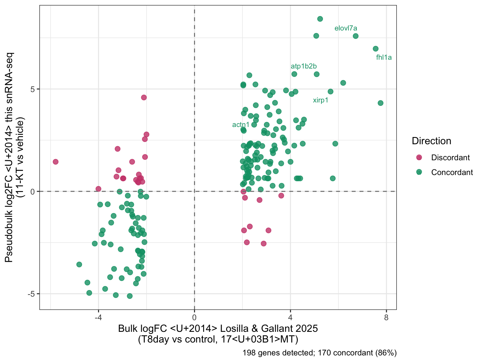
ImportantChallenge 3: Interpreting the cross-study comparison (15 min)
Use the scatter plot and concordance numbers to answer:
- Direction concordance. Is the rate substantially above 50% (random chance)? What does that say about whether Harmony + pseudobulk preserved the biological signal?
- Effect-size correlation. Do genes with large bulk logFC also show larger snRNA-seq fold-changes? What does a positive trend mean beyond direction alone?
- Hormone comparison. Losilla used 17α-methyltestosterone (17αMT); we used 11-KT. Both are androgens but differ in receptor selectivity and aromatization potential. Would you predict the same genes responding, a subset, or different ones?
TipSolution
- Concordance >70% is strong evidence that the androgen response was preserved. Because the studies used different androgens, different animals, and different sequencing technologies, high directional agreement provides cross-validation.
- A positive trend means relative effect sizes match across methods — not just direction but magnitude. Genes near the origin in both axes respond weakly in both; the upper-right and lower-left quadrants are robust hits.
- Most canonical androgen targets are expected to respond to both — both act through the androgen receptor. Differences could arise from (a) receptor selectivity — 11-KT is the physiological teleost androgen and may bind with higher affinity than synthetic 17αMT; (b) aromatization — 17αMT cannot be converted to estrogens, whereas 11-KT’s aromatization potential differs, possibly activating estrogen-receptor pathways selectively in one study.
TipKey Points
- Cluster markers from
FindAllMarkersplus NCBI gene-product descriptions are the bridge from cluster number to cell-type identity. - Curated marker gene lists from the EO literature, combined with
AddModuleScore, give defensible cell-type labels in a non-model organism. - A falsifiable prediction — the stalk should carry the post-synaptic NMJ apparatus (
musk/AChR) — beats labeling by exclusion: it points cleanly to the subsynaptic cluster (17) and is corroborated by the absent motor-neuron soma. - Nuclei from the same fish are not independent replicates; treating them as such is pseudoreplication and inflates false-positive rates.
- Pseudobulk aggregation (
AggregateExpressionwithassay = "RNA") sums raw counts per (cell-type × sample), restoring the n=2-per-group structure for DESeq2. - With n=2 per group, report log2FoldChange and direction first, padj second. Plot every fish — never group means.
- propeller (or arcsine-limma) tests cell-type proportion shifts; with n=2 it is severely underpowered and should be interpreted as a ranked list, not a hypothesis test.
- Direction concordance >50% with Losilla & Gallant 2025 — and a positive logFC–logFC correlation — confirms that the snRNA-seq pipeline preserved the biological androgen response.